How to Optimize Code¶

When considering the performance of code, the things to worry about in order of importance:

Algorithmic complexity.
Allocations and copies.
Memory access and cache performance.
Number of instructions.

Most programs will achieve acceptable performance by only considering the first two points, however, when doing computationally intensive tasks like the numeric programming required for quantitative finance, the 3rd and 4th point may become important.

Algorithmic Complexity¶

Algorithmic complexity is a measure of the relationship between input size and computation time.

Big-O: how code slows as data grows.

Ned Batchelder

The common technique for describing the time complexity of an algorithm is to compute the worst case performance of an algorithm. The standard way to communicate the worst case performance is through “Big O Notation”.

The intuition is to count the number of operations that happen for every element of the input. For example:

def contains(haystack, needle):
    for value in haystack:
        if value == needle:
            return True

    return False

In this example, for each element in haystack, we will perform 1 comparison, meaning there is a linear relationship between the time spent in contains and the length of haystack. This means that contains is \(O(n)\) with relation to haystack.

def contains_sorted(haystack, needle):
   while haystack:
       mid_ix = len(haystack) // 2
       midpoint = haystack[mid_ix]
       if midpoint == needle:
           return True
       if midpoint < needle:
           haystack = haystack[mid_ix + 1:]
       else:
           haystack = haystack[:mid_ix]
   return False

In this example, we cut the size of the haystack list in half in each step of the loop. This means that for a needle size of 16, in the worst case (the value is not in the haystack), we will operate on 16, 8, 4, 2, 1 values. This means we had 5 operations for 16 inputs. If we check 32, we will get 32, 16, 8, 4, 2, 1, or 6 operations. This function actually scales logarithmically with the size of haystack. This means that contains_sorted is \(O(ln(n))\) with relation to haystack.

The second function requires that the input is pre-sorted, but will perform much better for large haystacks given that constraint.

Reality Check¶

Algorithmic complexity is a good tool for quickly evaluating how an algorithm will scale as the data approaches infinity. However, in the real world, we are often working with finite data sets (even big data is finite). When working with finite data, it is important to remember the constants that get erased and the derivative of the scaling function.

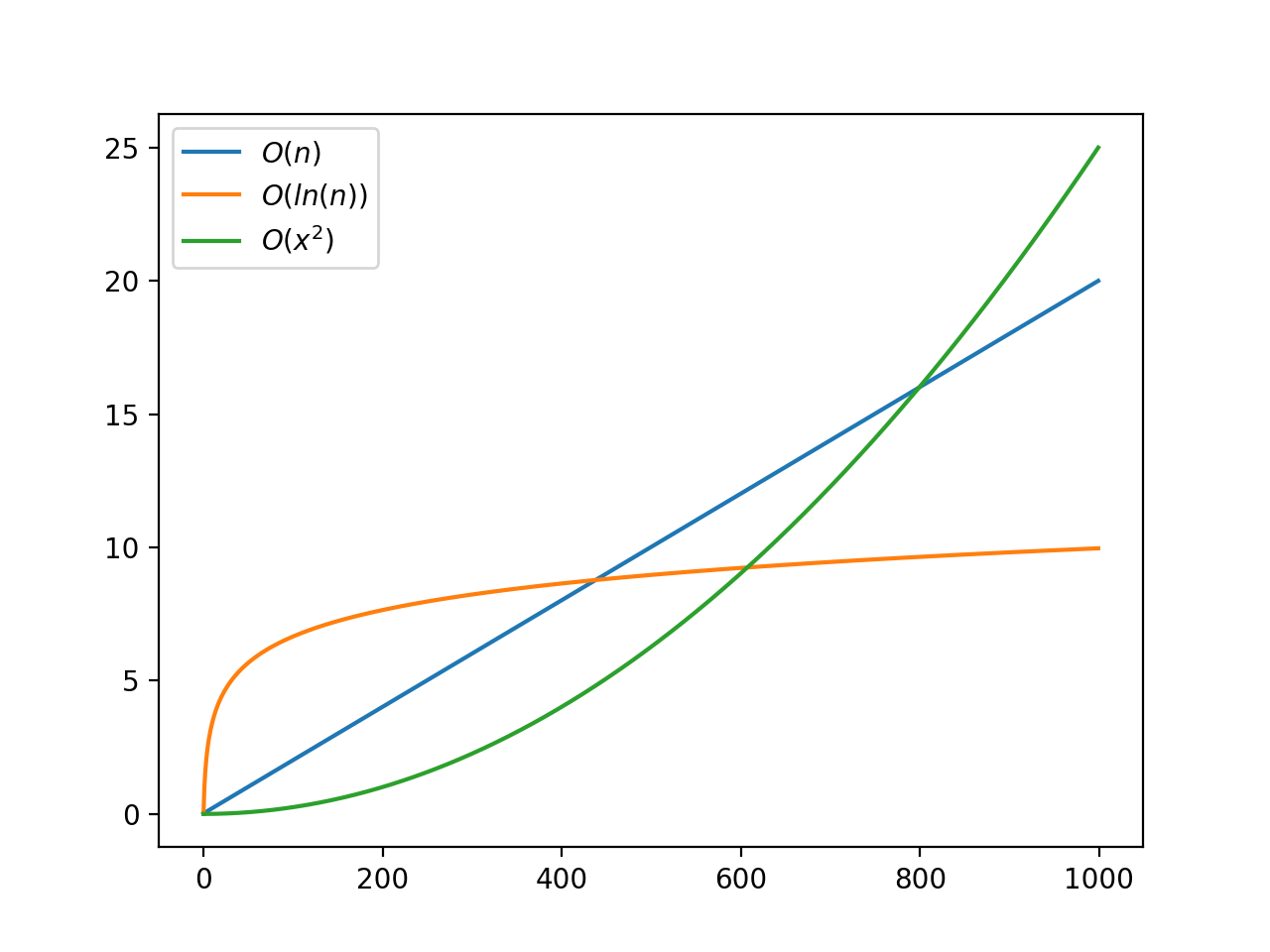
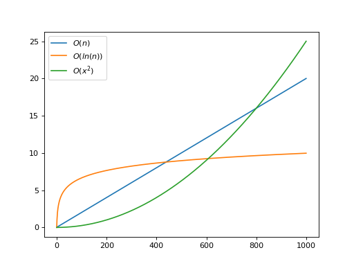
For example, here are three functions:

def f0(xs):
    for x in xs:
        pass

def f2(xs):
    for x in xs:
        pass

    for x in xs:
        pass

def f3(xs):
    # slow down, the data isn't going anywhere
    sleep(100)

The first function performs one operation, pass, per element. Therefore this function is linear. The second function performs 2 operations per element by looping twice so it is also linear. The third function performs 0 operations per element, so it has constant time scaling. This function will run in the same time regardless of the size of the input. However, the constant speed is 100 seconds, which may very well be slower than the linear solution for “small” xs.

This plot shows a linear function, a logarithmic function, and a quadratic function. Because of the particulars of these functions, the quadratic function would be faster until around 600 elements. If the expected input size was less than 600, then the quadratic algorithm would actually be the best choice!

(Source code, png, hires.png, pdf)

Allocations and Copies¶

Memory allocations can be very expensive. Allocating memory is itself potentially expensive because of the interaction with the operating system as well as the book keeping needed to track the newly allocated memory. The other, less obvious reason why allocations are bad is that it further spreads your data across more distinct addresses meaning you will get worse cache locality with the data.

Copies have all of the problems as allocations with the addition of an \(O(n)\) operation to traverse the values being copied. Scanning a large region of memory can evict the entire working set from the L1 cache because it is touching a lot of memory at once.

This isn’t to say that you shouldn’t allocate any memory. Programs sometimes need to store their results in new allocations; however, be careful about it.

The Fastest Operation¶

One of the most important tricks is to note that the fastest operation you can do is nothing. If you are struggling to improve the performance of some code, step back and think, “do I need to be doing this at all”. It can be easy to fall into the trap of optimizing a an algorithm as it exists, which may only be a locally optimal solution, when the globally optimal solution is to just call the function less times, or not at all.